Collections of Stereo Matching from KITTI

本文记录了 Stereo Matching 有文章/有code实现的主要paper.将会持续update

其中本站其他页面已有的文章为CSPN,AcfNet, CDN-GANet, DeepPruner, PSMNet, FADNet, SsSMnet, RTS2Net.

目录:

• Collections of Stereo Matching from KITTI
• GANet
• AANet
• DecomposeNet
• NVStereoNet
• STTR: Revisiting Stereo Depth Estimation From a Sequence-to-Sequence Perspective with Transformers
  • 整体结构
  • Optimal Transport

GANet

pdf code

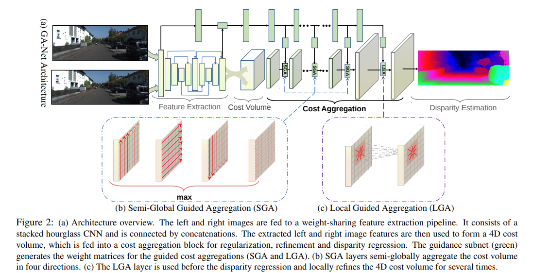
Feature Extraction使用的是stacked hourglass network. Cost Volume的形成与PSMNet一致。然后接数个SGA模块，以及LGA模块。左图会接上"guidance subnet"使用数个简单卷积生成权重矩阵提供到GA模块中。

GA层对应scanline optimization方法 ref1 ref2,可以理解为一个动态规划算法,其中本文的$\mathbf{r}$为四个方向的矢量。里面的权重是每一个像素不一致的，通过subnet提供guidance.

Semi-Global Guided Aggregation(SGA) 需要的guidence权重大小为$H\times W \times K\times F(K=5)$，不同disparity使用的权重一致: $$C_{\mathbf{r}}^{A}(\mathbf{p}, d)=\operatorname{sum}\left\{\begin{array}{l} \mathbf{w}_{0}(\mathbf{p}, \mathbf{r}) \cdot C(\mathbf{p}, d) \\ \mathbf{w}_{1}(\mathbf{p}, \mathbf{r}) \cdot C_{\mathbf{r}}^{A}(\mathbf{p}-\mathbf{r}, d) \\ \mathbf{w}_{2}(\mathbf{p}, \mathbf{r}) \cdot C_{\mathbf{r}}^{A}(\mathbf{p}-\mathbf{r}, d-1) \\ \mathbf{w}_{3}(\mathbf{p}, \mathbf{r}) \cdot C_{\mathbf{r}}^{A}(\mathbf{p}-\mathbf{r}, d+1) \\ \mathbf{w}_{4}(\mathbf{p}, \mathbf{r}) \cdot \max _{i} C_{\mathbf{r}}^{A}(\mathbf{p}-\mathbf{r}, i) \end{array}\right.$$ $$\text {s.t.} \quad \sum_{i=0,1,2,3,4} \mathbf{w}_{i}(\mathbf{p}, \mathbf{r})=1$$ $$C^{A}(\mathbf{p}, d)=\max _{\mathbf{r}} C_{\mathbf{r}}^{A}(\mathbf{p}, d)$$

Local Aggregation(LGA),需要的guidence权重大小为$H\times W\times 3K^2 \times F$: $$\begin{array}{c} C^{A}(\mathbf{p}, d)=\operatorname{sum}\left\{\begin{array}{l} \sum_{\mathbf{q} \in N_{\mathrm{p}}} \omega_{0}(\mathbf{p}, \mathbf{q}) \cdot C(\mathbf{q}, d) \\ \sum_{\mathbf{q} \in N_{\mathrm{p}}} \omega_{1}(\mathbf{p}, \mathbf{q}) \cdot C(\mathbf{q}, d-1) \\ \sum_{\mathbf{q} \in N_{\mathrm{p}}} \omega_{2}(\mathbf{p}, \mathbf{q}) \cdot C(\mathbf{q}, d+1) \end{array}\right. \\ \text { s.t. } \sum_{\mathbf{q} \in N_{\mathrm{p}}} \omega_{0}(\mathbf{p}, \mathbf{q})+\omega_{1}(\mathbf{p}, \mathbf{q})+\omega_{2}(\mathbf{p}, \mathbf{q})=1 \end{array}$$

AANet

pdf code

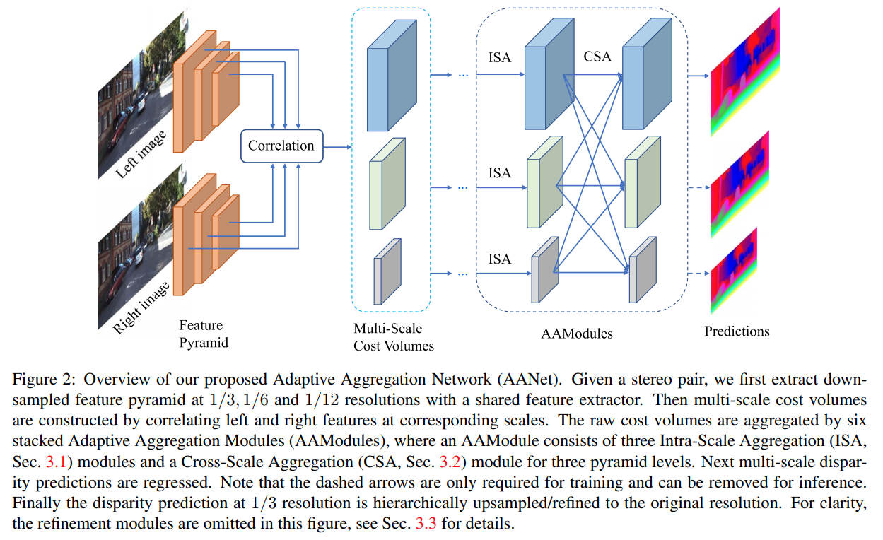
本文使用coorelation的方式生成3D Cost Volume.

Adaptive Intra-Scale Aggregation本质上是分组的可变卷积：

$$\tilde{\boldsymbol{C}}(d, \boldsymbol{p})=\sum_{k=1}^{K^{2}} w_{k} \cdot \boldsymbol{C}\left(d, \boldsymbol{p}+\boldsymbol{p}_{k}+\Delta \boldsymbol{p}_{k}\right) \cdot m_{k}$$

多scale融合，这里采用的是HRNet的方法 $$\hat{\boldsymbol{C}}^{s}=\sum_{k=1}^{S} f_{k}\left(\tilde{\boldsymbol{C}}^{k}\right), \quad s=1,2, \cdots, S$$

$$f_{k}=\left\{\begin{array}{l} \mathcal{I}, \quad k=s \\ (s-k) \text { stride }-2\oplus 3 \times 3 \text { convs, } \quad k<s \\ \text { upsampling } \oplus 1 \times 1 \text { conv, } \quad k>s \end{array}\right.$$

DecomposeNet

pdf

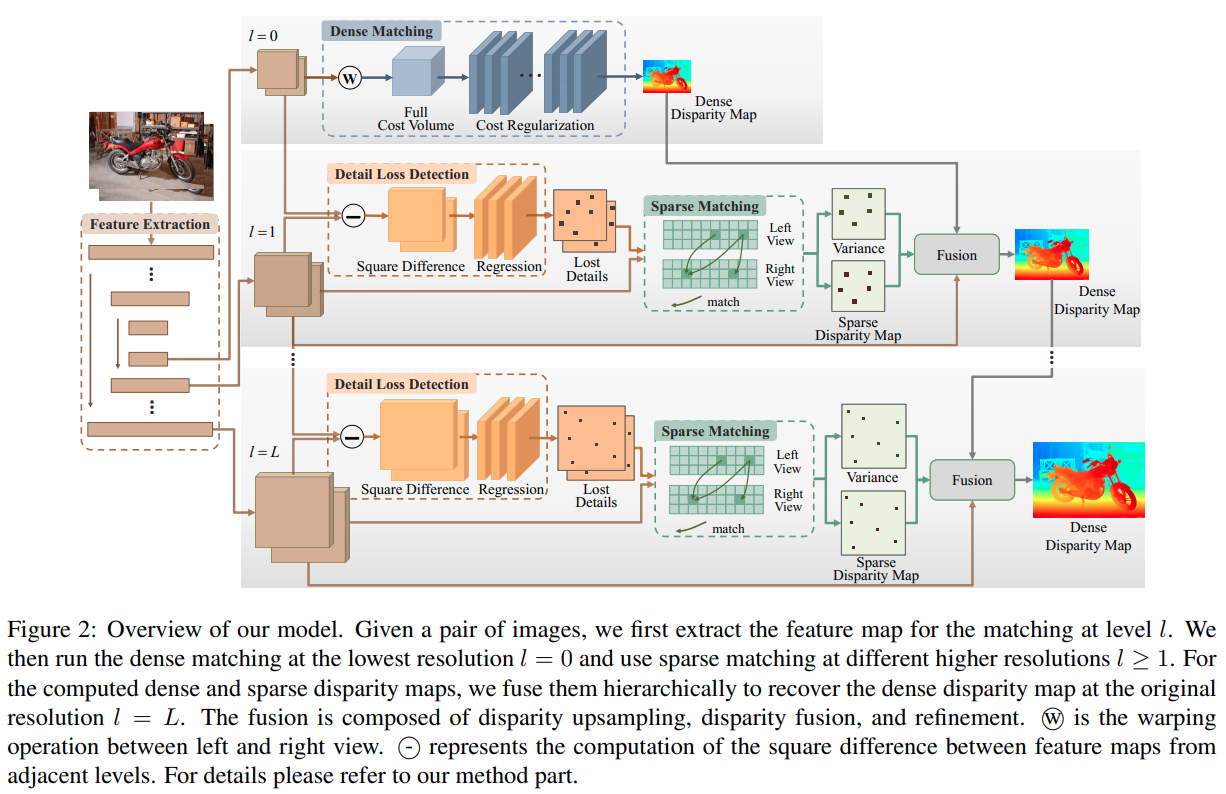
这篇paper的思路还是降低复杂度，在最低的分辨率下计算 Full Stereo Matching 的 Cost Volume. 在高分辨率下进行 Sparse Matching.

一张图概念上可以分为两种区域，一种是粗分类区域$CA$，这里的双目匹配结果可以从低分辨率上采样后refine出来；一种是细分类区域$FA$，这里的双目由高分辨率的sparse matching还原.

$$\begin{array}{c} \hat{D}_{L}=\widehat{\mathcal{F}}\left(\mathrm{FA}_{L}, \mathrm{FA}_{L}\right) \\ \vdots \\ \hat{D}_{1}=\widehat{\mathcal{F}}\left(\mathrm{FA}_{1}, \mathrm{FA}_{1}\right) \\ D_{0}=\mathcal{F}\left(\dot{\mathrm{A}}_{0}, \dot{\mathrm{A}}_{0}\right) \\ \tilde{D}=\hat{D}_{L} \cup \cdots \cup \hat{D}_{1} \cup D_{0} \end{array}$$

本文提出一个自监督的方案训练一个小网络识别图中被downsampling破坏的特征, 其输入是本层的特征$F_l$以及下层上采样的$F'_{l-1}$的特征差$F_l - F'_{l-1}$, 输出的网络可以被训练，训练目标是增加 $FA$区域的特征差，同时要求其稀疏.

$$\mathcal{L}_{l}^{\mathrm{DLD}}=\left|F A_{l}\right|-\alpha \frac{\sum_{(h, w) \in F A_{l}}\left\|F_{l}(h, w)-F_{l-1}^{\prime}(h, w)\right\|_{2}}{\left|F A_{l}\right|}$$

在稀疏Mask上直接计算disparity:

$$ \begin{aligned} C_{l}(h, w, d)&=<{F}{l}^{left}(h, w), {F}{l}^{right}(h, w-d)> \ P_{l}(h, w, d) &=\frac{\mathrm{e}^{C_{l}(h, w, d)-C_{l}^{\max }(h, w)}}{\sum_{d=0} \mathrm{e}^{C_{l}(h, w, d)-C_{l}^{\max }(h, w)}} \ C_{l}^{\max }(h, w) &=\max {d} C{l}(h, w, d) \

\hat{D}{l}(h, w)&=\sum{d=0} P_{l}(h, w, d) * d \end{aligned} $$

NVStereoNet

pdf code

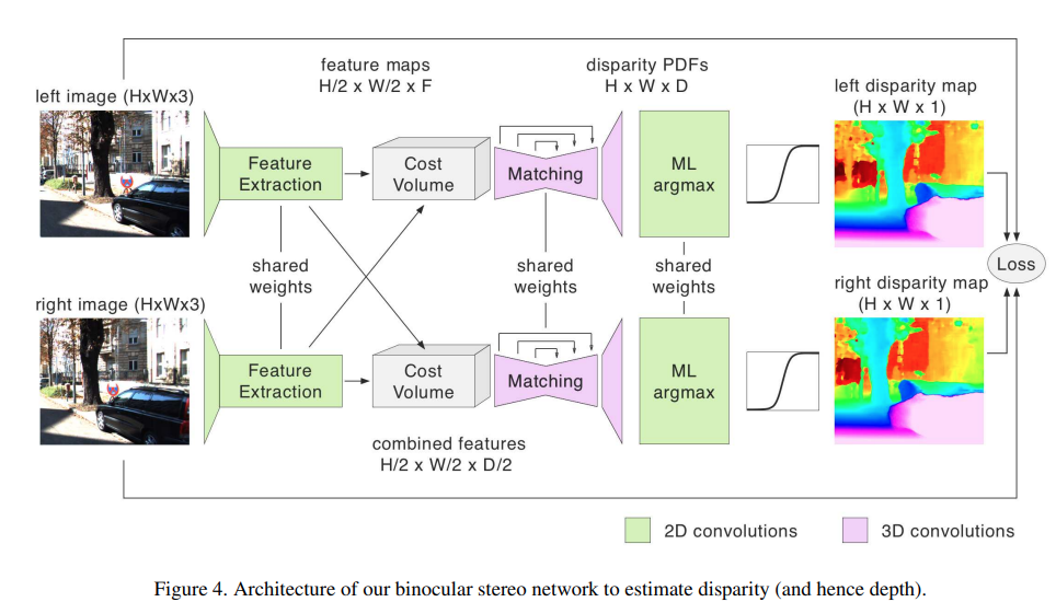
损失与monodepth相似

$$L=\lambda_{1} E_{\text {image}}+\lambda_{2} E_{\text {lidar}}+\lambda_{3} E_{l r}+\lambda_{4} E_{d s}$$

$$\begin{aligned} E_{\text {image}} &=E_{\text {image}}^{l}+E_{\text {image}}^{r} \\ E_{\text {lidar}} &=\left|d_{l}-\bar{d}_{l}\right|+\left|d_{r}-\bar{d}_{r}\right| \\ E_{l r} &=\frac{1}{n} \sum_{i j}\left|d_{i j}^{l}-\tilde{d}_{i j}^{l}\right|+\frac{1}{n} \sum_{i j}\left|d_{i j}^{r}-\tilde{d}_{i j}^{r}\right| \\ E_{d s} &=E_{d s}^{l}+E_{d s}^{r} \end{aligned}$$

$$\begin{aligned} E_{\text {image}}^{l} &=\frac{1}{n} \sum_{i, j} \alpha \frac{1-\operatorname{SSIM}\left(I_{i j}^{l}, \tilde{I}_{i j}^{l}\right)}{2}+(1-\alpha) | I_{i j}^{l}-\tilde{I}_{i j}^{l} \\ E_{d s}^{l} &=\frac{1}{n} \sum_{i, j}\left|\partial_{x} d_{i j}^{l}\right| e^{-\left\|\partial_{x} I_{i, j}^{l}\right\|}+\left|\partial_{y} d_{i j}^{l}\right| e^{-\| \partial_{y} I_{i, j}^{l}} \| \end{aligned}$$

STTR: Revisiting Stereo Depth Estimation From a Sequence-to-Sequence Perspective with Transformers

pdf code

这篇paper用Sequence/Transformer的角度重新理解双目pixel-wise matching. 作者指出主要有三大优势:

• 不再强约束要求一个固定的disparity上限
• 能识别遮挡区域，给出confidence
• 给出uniqueness约束 (这个是通过求解一个最优化问题实现的)

整体结构

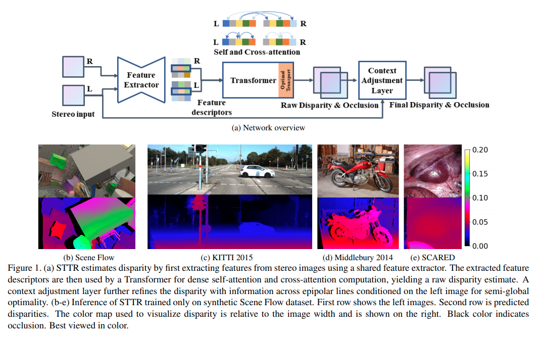
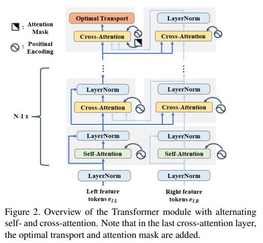
本文的网络结构的每一个部件都是基础部件，设计上或者代码上主要的不同点:

• backbone网络采用的是类似于U-Net的结构,但是在最后一层采样后加了一个DeepLabv3的ASPP
• multiheader transformer里面交错使用self-attention与cross attention.而代码上两者分别只有一个multi-head的ModuleList, 也就是图中重复的模块使用的是相同的参数.
• attention是先调整形状$[1, C, H, W] \rightarrow [H, W, C]$, 输出相当于是在$W$上展开一个个像素匹配，也就是理解为只在水平 epipolar line上进行匹配, 输出形状 $[H, W, W]$
• Position Embedding 采用的是作者提出的相对位置encode, 这个encoding是一个$[B, C, H, \times (2W-1)]$, 的encoder.
• 由于多层multihead的transformer运算量和显存占用很大，代码实现上需要用 checkpoint 技巧，也就是暂时不存储中间运算变量，在backward的时候再重新前传计算中间运算变量.
• 去到最后一层的时候作者指出应该考虑相机左右放置的关系，右feature与左feature计算attention的时候应该只计算部分的attention值 (上半三角).

Optimal Transport

从网络中得到$W \times W$匹配损失矩阵后，我们希望得到每一个像素的最优的, unique的结果. 这个问题可以被formulate为一个 optimal transport的问题, 有一个从分甜品motivate的比较好的博客. 用STTR这篇paper的语言进行问题表述:

$$\begin{aligned} \underset{\vec P}{\text{minimize}} \quad &\underset{i,j}{\sum}P_{ij} M_{ij} + \frac{1}{\lambda} \sum_{i,j} P_{i,j} \log P_{i,j} \\ \text{subject to} \quad & \sum_i P_{i,j} = c_j\\ & \sum_j P_{i,j} = r_i\\ \end{aligned}$$ 目标函数的第一项为由损失函数矩阵决定的线性函数，第二项为交叉熵。约束函数要求每一个左图的像素只会对应一个右图的像素(概率和为1)， 每一个右图的像素也只会对应一个左图的像素.

Optimal Transport是一个 凸优化中的LP问题，使用KKT条件中对$P$的导数为零可以得到: $$P_{ij} = \alpha_i \beta_j e^{-\lambda M}$$ 其中 $\alpha$和$\beta$与拉格朗日乘子和超参数$\lambda$有关，从约束中求解获得.

Sinkhorn Distances的原始代码则是:

def compute_optimal_transport(M, r, c, lam, epsilon=1e-8):
    """
    Computes the optimal transport matrix and Slinkhorn distance using the
    Sinkhorn-Knopp algorithm. From https://michielstock.github.io/OptimalTransport/

    Inputs:
        - M : cost matrix (n x m)
        - r : vector of marginals (n, )
        - c : vector of marginals (m, )
        - lam : strength of the entropic regularization
        - epsilon : convergence parameter

    Outputs:
        - P : optimal transport matrix (n x m)
        - dist : Sinkhorn distance
    """
    n, m = M.shape
    P = np.exp(- lam * M)
    P /= P.sum()
    u = np.zeros(n)
    # normalize this matrix
    while np.max(np.abs(u - P.sum(1))) > epsilon:
        u = P.sum(1)
        P *= (r / u).reshape((-1, 1)) # normalize in first dimension
        P *= (c / P.sum(0)).reshape((1, -1)) #normalize in second dimension
    return P, np.sum(P * M)

本文的代码则是默认$\lambda$为1，在 $\log$空间中进行迭代计算。